Fetching the Starbucks location dataset
The data can be found here at this Socrata portal, which is described as:
All Starbucks Locations in the World
An export of all Starbucks locations in the world. This dataset was scraped from the Starbucks website and is regularly updated.
Exporting the data and saving to our local drive as starbucks.csv
import requests
DATA_URL = 'https://opendata.socrata.com/api/views/xy4y-c4mk/rows.csv?accessType=DOWNLOAD'
resp = requests.get(DATA_URL)
with open("starbucks.csv", 'w') as f:
    f.write(resp.text)
Filter the data for US only
Assuming that starbucks.csv contains the full dataset, we create a filtered version by selecting only rows that have a country of "US" and removing unnecessary columns. The result of the below routine creates a new file named us-starbucks.csv:
HEADERS = ['City', 'Name', 'Latitude', 'Longitude', 'Store Number',
           'Street Combined', 'Postal Code', 'Country Subdivision',
           'Country', 'Ownership Type']
from csv import DictReader, DictWriter
with open("us-starbucks.csv", 'w') as w:
    dw = DictWriter(w, fieldnames = HEADERS)
    dw.writeheader()
    with open("starbucks.csv", 'r') as r:
        for row in DictReader(r):
            if row['Country'] == 'US':
                xo = {key: row[key] for key in HEADERS}
                dw.writerow(xo)
Calculating distance to nearest store for every store
This is the time-consuming stage.
Given that us-starbucks.csv contains all U.S.-based Starbucks locations.
For each Starbucks location, find the nearest Starbucks to it and calculate the distance in kilometers.
Another way to state this is: for every U.S. Starbucks location, sort the list of all U.S. Starbucks locations in ascending order of distance to the given location. Then add a new column/attribute named 'nearest_store_distance_km'.
The haversine function
How do we find the distance between any two given Starbucks? The haversine formula is a way to calculate distance between latitude and longitude points. This StackOverflow question has a nice explanation and implementation for Python: Haversine Formula in Python (Bearing and Distance between two GPS points)
What I've done below is create a function that takes arguments a and b and expects them both to be dictionaries with 'Longitude' and 'Latitude' keys, because I know each row in our dataset contains those key-value pairs:
def haversine_on_rows(a, b):
    from math import radians, cos, sin, asin, sqrt
    lon1 = radians(a['Longitude'])
    lon2 = radians(b['Longitude'])
    lat1 = radians(a['Latitude'])
    lat2 = radians(b['Latitude'])
    # haversine formula
    dlon = lon2 - lon1
    dlat = lat2 - lat1
    a = sin(dlat / 2) ** 2 + cos(lat1) * cos(lat2) * sin(dlon / 2) ** 2
    c = 2 * asin(sqrt(a))
    r = 6371 # Radius of earth in kilometers.
    # return the final calculation
    return c * r
Assuming that we're starting in a fresh Python session/script, and the above function has been interpreted, let's set the variables and requirements:
HEADERS = ['City', 'Name', 'Latitude', 'Longitude', 'Store Number',
           'Street Combined', 'Postal Code', 'Country Subdivision',
           'Country', 'Ownership Type',
           "nearest_store_number", "nearest_store_distance_km"]
from csv import DictReader, DictWriter
Preprocessing the deserialized store data
To get the store data, we just read in us-starbucks.csv as a CSV file. However, I do a little preprocessing. Remember that CSV files (unlike JSON), because they're just plaintext values separated by commas, deserialize all values as strings – it doesn't assume that a number value is actually a number.
So in the routine below, I create a new list named drows and for each row (dictionary) in the dataset, I manually convert Longitude and Latitude to floats, then append it to the drows list. That saves me from having to do string-to-float conversions later on (i.e in the haversine function).
drows = []
with open("us-starbucks.csv", 'r') as rf:
    for row in DictReader(rf):
        row['Longitude'] = float(row['Longitude'])
        row['Latitude'] = float(row['Latitude'])
        drows.append(row)
with open("us-starbucks-distant.csv", 'w') as w:
    dw = DictWriter(w, fieldnames = HEADERS)
    dw.writeheader()

    for i, row in enumerate(drows):
        # assuming the nearest row distance is 0, the store compared to itself
        # we assume the next row contains the actual nearest store
        n_row = sorted(drows, key=lambda x: haversine_on_rows(row, x))[1]
        row['nearest_store_number'] = n_row['Store Number']
        # redundant calculation but oh well
        row['nearest_store_distance_km'] = round(haversine_on_rows(row, n_row), 1)
        print(i, row['nearest_store_distance_km'])
        print("\t", row['City'], row['Country Subdivision'], row['Name'])
        print("\t", n_row['City'], n_row['Country Subdivision'], n_row['Name'])
        dw.writerow(row)
You can download my filtered CSV here.
Get a quick report
Now that the us-starbucks-distant.csv file has been created, we can read it, sort it by the nearest_store_distance_km column, and get a quick list of the top 10 most isolated Starbucks:
from csv import DictReader
with open("us-starbucks-distant.csv", 'r') as r:
    rows = sorted(DictReader(r),
                  key=lambda x: float(x['nearest_store_distance_km']),
                  reverse=True)

print("The 10 most isolated Starbucks in America are:")
for i, row in enumerate(rows[0:10]):
    print("%s. %s km -- %s, %s (%s)" % (str(i + 1).rjust(2),
                         row['nearest_store_distance_km'].rjust(5),
                         row['City'],
                         row['Country Subdivision'],
                         row['Name']))
The output:
The 10 most isolated Starbucks in America are:
 1. 377.5 km -- Ketchikan, AK (Carrs-Ketchikan #1818)
 2. 209.3 km -- Kodiak, AK (Safeway-Kodiak #1090)
 3. 183.2 km -- Del Rio, TX (Veterans & Chevrolet)
 4. 165.7 km -- Page, AZ (Safeway - Page #249)
 5. 155.1 km -- Garden City, KS (Target Garden City T-906)
 6. 155.1 km -- Colby, KS (Oasis Travel Center)
 7. 151.2 km -- Dickinson, ND (Family Fare - Dickinson #3123)
 8. 149.7 km -- Hays, KS (Fort Hays State University)
 9. 147.7 km -- North Platte, NE (North Platte-I80 & S Hwy 83)
10. 145.4 km -- Gallup, NM (Safeway-Gallup #1743)
Create a Google Static Map
The Google Static Maps API lets us create a URL that points to a map image with custom markers. We'll follow the same strategy above and create markers letter A through J to mark the most isolated Starbucks in descending order.
from urllib.parse import urlencode
from csv import DictReader
from string import ascii_uppercase
with open("us-starbucks-distant.csv", 'r') as r:
    rows = sorted(DictReader(r),
                  key=lambda x: float(x['nearest_store_distance_km']),
                  reverse=True)[0:10]

markers = []
for i, row in enumerate(rows):
    letter = ascii_uppercase[i]
    markers.append("label:" + letter + '|' + row['Latitude'] + ',' + row['Longitude'])

gmap_url = 'https://maps.googleapis.com/maps/api/staticmap'
myparams = {'size': '800x400', 'markers': markers}
query_str = urlencode(myparams, doseq=True)
print(gmap_url + '?' + query_str)
The resulting URL:
https://maps.googleapis.com/maps/api/staticmap?size=800x400&markers=label%3AA%7C55.34944534301758%2C-131.673828125&markers=label%3AB%7C57.81049346923828%2C-152.36724853515625&markers=label%3AC%7C29.392152786254883%2C-100.90473937988281&markers=label%3AD%7C36.915977478027344%2C-111.4585189819336&markers=label%3AE%7C37.98002624511719%2C-100.84310150146484&markers=label%3AF%7C39.36470031738281%2C-101.05500030517578&markers=label%3AG%7C46.87602233886719%2C-102.79847717285156&markers=label%3AH%7C38.8739128112793%2C-99.34193420410156&markers=label%3AI%7C41.115745544433594%2C-100.76504516601562&markers=label%3AJ%7C35.53567886352539%2C-108.75711059570312
Which looks like this:

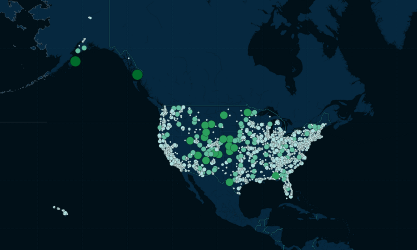
CartoDB
This is as simple as just uploading into CartoDB. You can see my finished map here.
Here's a screenshot of that map: